Forward and Reverse Mode Differentiation
Summary
Methods to efficiently compute gradients are important as gradients underpin the training of machine learning models. In this article, we will compare forward and backward mode differentiation for gradients of function compositions.
This is particularly relevant to Neural Networks where the ubiquitous backpropagation algorithm is simply backward mode differentiation. Its forward counterpart has historically been ignored as it runs too slowly. However, backward mode requires more memory and memory limitations are now emerging as a concern. In order to work with larger models, practitioners must address the classical Time-Space tradeoff.
Background
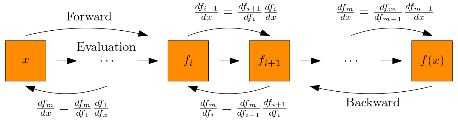
Given functions $f_{0}(x) := x$ and $f_{1}, \dots, f_{m}$ with known Jacobians, we want to compute the Jacobian of their composition
\[f(x) = f_{m} \circ \cdots \circ f_{1} (x),\quad f_{i}:\mathbb{R}^{d_{i-1}} \to \mathbb{R}^{d_{i}}.\]By the Chain Rule,
\[\underset{ d_{m} \times d_{0} }{ \frac{df}{dx} \vphantom{\frac{df_{m}}{df_{m-1}}} } = \underset{ d_{m} \times d_{m-1} }{ \frac{df_{m}}{df_{m-1}} \vphantom{\frac{df_{m}}{df_{m-1}}} } \cdots \underset{ d_{1} \times d_{0} }{ \frac{df_{1}}{df_{0}} \vphantom{\frac{df_{m}}{df_{m-1}}} } = \prod_{i=1}^{m} \frac{df_{i}}{df_{i-1}}.\]We refer to each term in the product as a transition Jacobian.
Jacobian
Recall that Jacobian of $f : \mathbb{R}^{d_{0}} \to \mathbb{R}^{d_{m}}$ is defined as $$ \left(\frac{df}{dx}\right)_{ij} = \frac{\partial f_{i}}{\partial x_{j}},\quad \frac{df}{dx} = \underset{ d_{m} \times d_{0} }{ \begin{bmatrix} \vdots & \vdots & \vdots \\ \frac{\partial f}{\partial x_{1}} & \cdots & \frac{\partial f}{\partial x_{d_{0}}} \\ \vdots & \vdots & \vdots \end{bmatrix}. } $$ See Notation section at end of page for clarification on what is meant by $\frac{df_{i}}{df_{i-1}}$.
Now it remains to establish a scheme to compute $\frac{df}{dx}$ efficiently. We follow Appendix A.1 from (Kidger, 2022) for details.
Forward Mode Differentiation
This method studies how the intermediate layers $f_{i}$ vary with the initial layer $x$. We apply a forward recursion until we obtain the Jacobian of the final layer $f$.
Forward Mode Recursion
For $i = 0, \dots, m-1$, $$ \underset{ d_{i+1} \times d_{0} }{ \frac{df_{i+1}}{dx} \vphantom{\frac{df_{i+1}}{df_{i}}} } = \underset{ d_{i+1} \times d_{i} }{ \frac{df_{i+1}}{df_{i}} \vphantom{\frac{df_{i+1}}{df_{i}}} } \, \underset{ d_{i} \times d_{0} }{ \frac{df_{i}}{dx} \vphantom{\frac{df_{i+1}}{df_{i}}} }. $$
The algorithm comprises of one pass which computes $f(x)$ and $\frac{df}{dx}$
- Base Case $f_{0} = x$ and $\frac{df_{0}}{dx} = I$ (Identity matrix)
- Iteration $i$:
- Recall $x_{i}$ and $\frac{df_{i}}{dx}$ from the previous iteration
- Compute $x_{i+1} = f_{i+1}(x_{i})$ and transition Jacobians $\frac{df_{i+1}}{df_{i}}(x_{i})$
- Compute $\frac{df_{i+1}}{dx} = \frac{df_{i+1}}{df_{i}} \frac{df_{i}}{dx}$
- Set $i = i + 1$
- At iteration $m$, return $\frac{df_{m}}{dx}$
Backward Mode Differentiation
This method studies how the output $f$ varies with the intermediate layers $f_{i}$. We apply a backward recursion until we obtain the Jacobian with respect to the initial layer $x$.
Backward Mode Recursion
For $i = 0, \dots, m-1$, $$ \underset{ d_{m} \times d_{m-i-1} }{ \frac{df_{m}}{df_{m-i - 1}} \vphantom{\frac{df_{m}}{df_{m-i}}} } = \underset{ d_{m} \times d_{m-i} }{ \frac{df_{m}}{df_{m-i}} \vphantom{\frac{df_{m}}{df_{m-i}}} } \; \underset{ d_{m-i} \times d_{m-i-1} }{ \frac{df_{m-i}}{df_{m-i-1}} \vphantom{\frac{df_{m}}{df_{m-i}}} }. $$
The algorithm comprises two passes.
- The forward pass computes and stores all$f_{i}$
- Same as forward mode but we do not compute the transition Jacobians
- The backward pass computes $\frac{df_{m}}{dx}$.
- Base case $\frac{df_{m}}{df_{m}} = I$
- At iteration $i$:
- Evaluate the transition Jacobian $\frac{df_{m-i}}{df_{m-i-1}}$ using $f_{m-i-1}$ as input
- Compute $\frac{df_{m}}{df_{m-i-1}} = \frac{df_{m}}{df_{m-i}} \frac{df_{m-i}}{df_{m-i-1}}$
- Set $i = i + 1$
- At iteration $m$ return $\frac{df_{m}}{df_{0}} = \frac{df_{m}}{dx}$
Comparison
The direction of recursion in forward and backward mode yields the method’s name but it also results in the cost being dependent on the input and output dimensions respectively. In general, a recursion comprises matrix-matrix multiplication which is $O(d^{3})$ where $d = \max d_{i}$. However
- If $d_{0} = 1$ and $x$ is a scalar, then forward recursion comprises of a matrix-vector multiplication, $O(d^{2})$
- Likewise, if $d_{m} = 1$ and $f$ is a scalar, then backward recursion comprises vector-matrix multiplication, also $O(d^{2})$.
In the context of Neural Networks, $f$ typically corresponds to a scalar / 1D loss function (e.g. cross-entropy for classification and mean-squared error in regression). Hence, this is the case we will consider.
Computational-Cost
In terms of function evaluations and computation of transition Jacobians, forward and backward modes are identical. Hence, we only need to consider the cost of the recursion.
For forward mode, this is $O(md^{3})$ whereas only having to perform vector-matrix multiplication reduces the complexity of backward mode to $O(md^{2})$.
Numerical Stability
This discrepancy in computational cost is closely related to the common trick used in numerical linear algebra where $ABx$ is evaluated as $A(Bx)$ as opposed to $(AB)x$.
The other reason this is beneficial is that matrix-vector multiplication is numerically (backward) stable whereas matrix-matrix multiplication is not, see (Nakatsukasa, 2023, chap. 7.6). This means that a naive implementation of forward mode would be unstable. (It is possible to recover stability for an increased computational cost, see (Demmel et al., 2007). But in practice, the increase in computing time would exacerbated by a difference in software as it is relatively new.)
These two reasons demonstrate why backward mode is appealing. However, the next section outlines its major drawbacks.
Memory Cost
In forward mode, we only need to store the previous partial evaluation $f_i$ and compute the transition Jacobian. On the other hand, backward mode needs to store all the partial evaluations during the forward pass as it can only use them during the backward pass. Both need to use a transition Jacobian $O(d^{2})$. But with regards to partial evaluations, the cost is $O(d), O(md)$ respectively. (We exclude the cost of storing the transition Jacobian as in practice the vector-matrix product is computed directly which may not necessitate storing the Jacobian fully.)
As the increase in computational capabilities is plateauing, bandwidth limitation (the speed at which we can call stuff from memory) now poses as the bottleneck. (While a Neural Network like ResNet-50 requires 7.5 GB of data, this needs to be stored “close” together to ensure the latency of a memory request is low.) See (Graphcore, 2017).
There have been some attempts to alleviate this.
- Memory-Efficient Backpropagation Through Time (Gruslys et al., 2016)
- Proposed a method that decreased memory usage by 95% for backpropagation in a recurrent neural network.
- For recurrent neural networks, because the depth $m$ is large, the memory cost is acutely felt.
- The Symplectic Adjoint Method: Memory-Efficient Backpropagation of Neural-Network-Based Differential Equations (Matsubara et al., 2023)
- Neural-Based Differential Equation refers to $du = f_{\theta}(u) dt$ where $f_{\theta}$ is a neural network.
- Evaluating $u$ can be done through numerical integration which requires evaluation of $f_{\theta}$ say $n$ times. As we need to combine these values, we need to hold $O(nmd)$ in memory.
- The adjoint method only requires $O(md)$ memory but is numerically unstable.
- Their method is numerically stable while retaining the memory requirements of the adjoint method at the expense of increased computational cost.
These two papers indicate that memory cost is becoming a critical consideration in the design of algorithms. Often memory requirements are reduced by increasing computational cost.
Conclusion
Forward mode computes gradients while it evaluates the function $f$ whereas backward mode computes gradients in reverse after evaluation. Since $f$ is typically a scalar, forward mode takes longer to run whereas backward mode requires more memory.
In the past, the speed of training neural networks has been the main concern. The application of the backpropagation algorithm and advances in GPU-acceleration were necessary to demonstrate the feasibility of Neural networks, see AlexNet (Wikipedia, 2023). However, memory limitations are now emerging as a concern and practitioners will need to find a way to balance the classical Time-Space tradeoff.
| Mode | Computation | Memory | Stability |
|---|---|---|---|
| Forward | $O(md^{3})$ | $O(d)$ | Unstable |
| Backward | $O(md^{2})$ | $O(md)$ | Stable |
Table 1. Cost and stability summary of forward and reverse mode differentiation.
References
- Kidger, P. (2022). On Neural Differential Equations. arXiv. http://arxiv.org/abs/2202.02435
- Nakatsukasa, Y. (2023). Numerical Linear Algebra. University of Oxford. https://courses.maths.ox.ac.uk/course/view.php?id=5024#section-1
- Demmel, J., Dumitriu, I., & Holtz, O. (2007). Fast linear algebra is stable. Numerische Mathematik, 108(1), 59–91. https://doi.org/10.1007/s00211-007-0114-x
- Graphcore. (2017). Why is so much memory needed for deep neural networks? https://www.graphcore.ai/posts/why-is-so-much-memory-needed-for-deep-neural-networks
- Gruslys, A., Munos, R., Danihelka, I., Lanctot, M., & Graves, A. (2016). Memory-Efficient Backpropagation Through Time. arXiv. http://arxiv.org/abs/1606.03401
- Matsubara, T., Miyatake, Y., & Yaguchi, T. (2023). The Symplectic Adjoint Method: Memory-Efficient Backpropagation of Neural-Network-Based Differential Equations. IEEE Transactions on Neural Networks and Learning Systems, 1–13. https://doi.org/10.1109/TNNLS.2023.3242345
- Wikipedia. (2023). AlexNet — Wikipedia, The Free Encyclopedia. http://en.wikipedia.org/w/index.php?title=AlexNet&oldid=1182803102
Notation
As an example, let us take $m=3$ where $f = f_{3} \circ f_{2} \circ f_{1} \circ x$ and let us use $x_{i} \in \mathbb{R}^{d_{i-1}}$ as a dummy variable to represent the input of $f_{i}$. Formally, the Chain Rule is stated as
\[\left. \frac{df}{dx} \right \rvert_{x} = \left. \frac{df_{3}}{dx_{3}} \right \rvert_{x_{3} = f_{2} \circ f_{1} \circ x} \left. \frac{df_{2}}{dx_{2}} \right \rvert_{x_{2} = f_{1} \circ x} \left. \frac{df_{1}}{dx_{1}} \right \rvert_{x_1 = x}.\]This is notationally burdensome and by abuse of notation,
\[\frac{df}{dx} = \frac{df_{3}}{df_{2}} \frac{df_{2}}{df_{1}} \frac{df_{1}}{dx}.\]Nevertheless, it is suitable as our evaluation point is an evaluation of $f_{i-1}$ and hence has the correct dimension and value.